📓 JupyterLab¶

JupyterLab is a first-class way to drive the solver, not just a place to export a notebook. Once a scene has been transferred, the same project can be simulated, previewed, inspected, and iterated on entirely from a notebook on the solver host. Blender itself does not have to stay open: you can quit it, run the full simulation from JupyterLab, relaunch Blender later, and fetch the finished animation back onto the original meshes.

This page covers the whole loop in one place.

When to Reach for JupyterLab¶

Headless simulation. You have a laptop that you need to close, but the solver host can keep running. Export, quit Blender, and drive app.session.run() from a notebook that stays alive on the server.
Parameter sweeps and variant generation. Scripting solver.param / solver.session.param edits in a notebook is faster than clicking through the sidebar, and the results stream back as plots instead of viewport redraws.
Inspecting the codebase. The notebook attaches to the same frontend package the add-on talks to, so you can poke at app.scene, app.session, app.session.param, the fixed-scene report, and the live solver state interactively. It is a much faster way to learn the API than reading source, and a convenient surface for summarizing what a project contains.
Long runs you want to leave unattended. Kick off app.session.run() in a notebook cell, close the browser tab, and reconnect later to app.session.stream() the tail of stdout.

The End-to-End Loop¶

Sequence diagram with three lanes. Blender (1) on the left transferring and exporting to JupyterLab, then quitting; JupyterLab in the middle running app.session.run / preview / stream while frames land on disk; Blender (2) on the right launching later and pulling the animation back via Connect and Fetch — The three-lane loop. The first Blender session transfers the scene, exports the notebook, and optionally starts the solver, then quits. JupyterLab drives `run() / preview() / stream()` on the solver host while frames land on disk. A later Blender session launches, reconnects, and fetches the animation back onto the original meshes.¶

The thing that makes this work is the solver’s on-disk project state: mesh / param pickles from Transfer, plus whatever frames the solver has produced. As long as those live on the solver host, it does not matter whether Blender, JupyterLab, or neither is currently attached.

Note

You do not have to switch to JupyterLab just to leave a run unattended. A simulation launched from the Blender add-on Run button also survives Disconnect and even quitting Blender; reconnect later and Fetch All Animation to pull the frames. See Disconnecting while a simulation runs. Reach for JupyterLab when you want to drive the run (parameter sweeps, live previews, interactive inspection), not just step away.

Prerequisites¶

JupyterLab running and reachable from the add-on, by convention on the solver host, on the JupyterLab Port (default 8080).
A live connection: Connect plus Start Server on the main panel.
At least one Transfer into the current session so the notebook has something to attach to. Without it, BlenderApp.open(...) has no pickles to recover from.

The Jupyter Row¶

The main panel’s JupyterLab section has three buttons:

Button	What it does
Export	Write the template notebook onto the solver host
Open	Open `http://localhost:<port>/lab/tree/<path>` in your browser
Delete	Remove the notebook file from the solver host

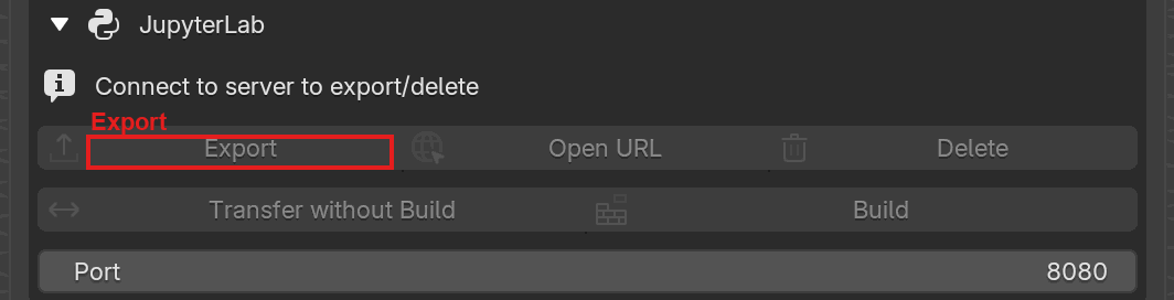
JupyterLab section inside the Solver panel — The JupyterLab section, expanded. The **Export** button writes the notebook onto the solver host. **Open URL** points the browser at it once an export exists, and **Delete** removes the server-side file.¶

Export pops a dialog for the target path. The default is blender-export/<project_name>.ipynb (or whatever you exported last). The filename must end with .ipynb. Writes go through the solver connection, not through Jupyter’s REST API.

Open is enabled once an export exists. It does not check that the file still exists on the server; if you deleted it manually, you will get a 404 in the browser.

Delete removes the server-side file and clears the add-on’s record of the last export, which disables Open again.

The Generated Notebook¶

Three cells, all Python:

Banner comment naming the project, so the notebook is self-identifying when shared.
Attach:
```
from frontend import BlenderApp

app = BlenderApp.open("<project>")
app.scene.report()
app.scene.preview()
```
BlenderApp.open(...) recovers a built scene if one is available; otherwise it populates and builds from the uploaded mesh and parameters. It is a no-op if the scene is already built, so running this cell repeatedly is safe.
Run:
```
app.session.run()
app.session.preview()
app.session.stream()
```
run() starts the solver (or attaches to an existing run, which is useful if you kicked it off from the add-on already). preview() gives a live frame playback widget, stream() tails stdout in realtime. To pick up a saved state instead, call app.session.resume() explicitly.

Note

The notebook’s BlenderApp comes from the solver repo’s frontend package, not the add-on. The add-on only writes the file.

Simulating Entirely from JupyterLab¶

Once the notebook is open, Blender is no longer required. A typical “quit Blender and simulate in the notebook” session looks like this:

In Blender, finish scene setup, Transfer, then Export notebook. Optionally press Start Server so a solver is already warm; if not, the notebook will spawn one when run() is called.
Open the notebook in your browser. Confirm the attach cell brings up the expected scene via app.scene.report() and app.scene.preview().
Quit Blender. The solver host keeps the pickles and any running server process; closing Blender only drops the add-on’s live connection.

From the notebook, run the simulation:

app.session.run()        # or app.session.resume() to continue
app.session.preview()    # live frame widget in the notebook
app.session.stream()     # tail solver stdout inline

Iterate in place. You can tweak parameters through app.session.param.* (see the JupyterLab Python API) and re-run without re-exporting. Because the notebook attaches to the pickled scene on disk, you can close the browser tab and reopen it later. The cell outputs may be gone, but rerunning the attach cell puts you right back where you were.

Returning to Blender and Fetching¶

When the run is done (or whenever you want the animation back on your Blender meshes):

Launch Blender and reopen the .blend you transferred from.
Connect to the same solver host. The session ID baked into the scene is how the add-on recognizes it is the same run.
Press Fetch All Animation. The add-on downloads the frames the JupyterLab run produced and wires the downloaded PC2 files up to each simulated mesh, exactly as if Blender had driven the run itself.
Scrub the timeline to confirm, then optionally Bake (see Baking Animation) to turn the fetched animation into plain Blender data.

Tip

If the reopened .blend warns about a session mismatch, it means the solver host has a different session stamped than your .blend remembers. Either reconnect to the run you actually want (matching session), or accept the mismatch if you are deliberately attaching to a new one; see Simulating → Sessions and recovery.

Inspecting the Codebase from a Notebook¶

The same notebook is a very natural place to explore what the solver understands about a project. Useful idioms:

app.scene.report()                       # group summary, counts, flags
app.scene.preview()                      # 3D preview of the fixed scene
app.session.param                         # live param object; tab-complete it
help(app.session)                         # frontend Session API surface
app.session.param.dyn("gravity")          # dynamic-parameter builder

Because frontend is just a Python package, inspect.getsource(...), ?? magics, and regular dir() all work. This makes a notebook a good place to summarize a project (what groups exist, what pins are bound, what parameters are in play) without clicking through every sidebar section in Blender.

Tips¶

Re-export after major scene changes. The notebook’s BlenderApp.open(...) picks up whatever pickles are on disk at the time the cell runs, so you normally do not need to re-export just to iterate on parameters. Re-export when you add or remove objects, rebuild groups, or change the project name.
Repeated exports overwrite. The filename is derived from the project name, so hitting Export twice is safe.
Delete to tidy up. Useful when flipping between experiments so stale .ipynb files do not accumulate under blender-export/.
If Open goes to the wrong port, the add-on uses the JupyterLab Port from scene state. Adjust it in the Jupyter preferences row, not via the URL.
Headless-friendly. run(), preview(), and stream() all work with Blender closed; the notebook does not depend on Blender’s Python at all.